This simple tutorial explains how to create a customized schedule that links wall objects in a drawing to a database worksheet. The schedule will display data for wall areas, wall thicknesses, labor cost, material cost, taxes, and total cost per wall style.
The WorksheetTutorial.vwx file contains the data required to perform the tutorial steps. Though wall styles are a Vectorworks Design Series feature, any Vectorworks license can use the wall styles that already exist in the tutorial file. Download the file here (internet access required) and open it in Vectorworks to begin.
There are three ways to create a schedule using worksheets. This tutorial uses the first option below.
● Start with a blank worksheet, and create the schedule from scratch. See Creating a Blank Worksheet.
● Create a schedule based on a common record format of a set of objects (wall data, in this example). This option allows you to select the criteria you wish to display from all the available object criteria. See Creating Reports.
● Start with a preformatted schedule and customize it to achieve your goals. See Using Preformatted Schedules.
To create a blank worksheet:
From the Resource Manager, click New Resource, select Worksheet, and then click Create. The Create Worksheet dialog box opens.
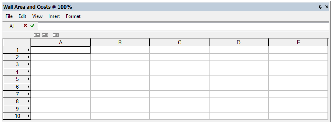
Enter “Wall Area and Costs” as the name for the new worksheet, and click OK. You will add more rows and columns later.
A blank worksheet window opens.
Next, create a database of the objects in the drawing from which to extract the wall area data. You can combine multiple criteria to collect the desired subset of objects.
For this tutorial, a single database of wall objects will be created and limited to a specified set of wall styles.
An alternative would be to create one database per wall style and include multiple databases in the same worksheet. However, for very large databases, it is recommended to create separate worksheets rather than include multiple databases into a single worksheet.
To set the database criteria:
Right-click (Windows) or Ctrl-click (Mac) on the header box for row 3.
From the Row context menu, select Database. The Criteria dialog box opens.
Set the three criteria options as follows:
● Type
● is
● Wall
Click More Choices, and set the next three criteria as follows:
● Wall Style
● is
● Aspen Interior Walls
Click More Choices, and set the next three criteria as follows:
● Wall Style
● is
● Ext-CIP Conc 36”-Footing
To include all wall styles in the schedule, do not enter criteria for walls and wall styles; instead, use the following criteria: Record, Wall Data, is present.
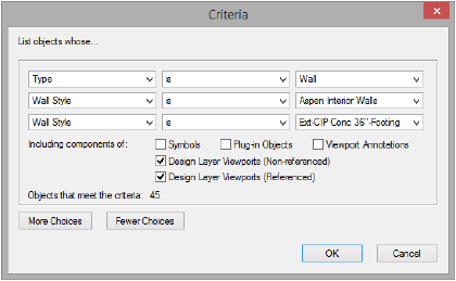
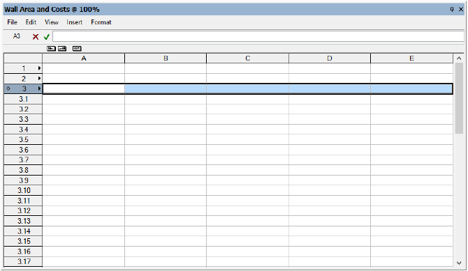
Click OK to set the criteria. The database of walls for the specified set of wall styles is created. The database header (row 3) now has a diamond next to the row number. Beneath row 3 are sub-rows for each object in the database (3.1 through 3.45).
For this tutorial, you need to expand the worksheet. Since no data has been assigned to the columns yet, it does not matter where the columns are added.
Use one of the following methods to add three columns to the worksheet, for a total of eight.
● Select Insert > Columns. An empty column is added to the left of the current column.
● Right-click (Windows) or Ctrl-click (Mac) the column header where you want to add a column, and select Insert Columns from the context menu.
● Position the cursor at the bottom right corner of the worksheet to activate a special resize cursor; drag to add columns to the right side of the worksheet.
Next, add database functions to the worksheet to extract the desired data from the database. Enter formulas for each column in the database header row cells. The database header row can be hidden before the worksheet is placed on the drawing.
For this tutorial, the following data will be extracted:
● Wall Style Name
● Gross Wall Area
● Net Wall Area
● Wall Thickness
To extract the data associated with the walls in the database:
Click the following cells and enter the formula shown to extract data for each item in the database. Be sure to include the equal sign (=) before each item.
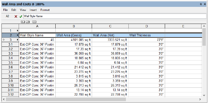
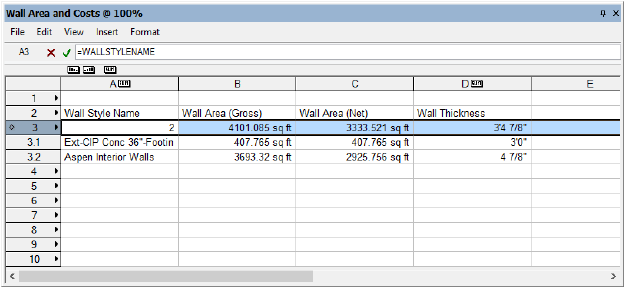
● In A3 enter =WALLSTYLENAME
● In B3 enter =WALLAREA_GROSS
● In C3 enter =WALLAREA_NET
● In D3 enter =WALLTHICKNESS
Alternatively, use the worksheet menu command Insert > Function to insert functions.
By default, numerical data is unformatted and must be formatted to display appropriate units. Formatting applied to database header row cells is automatically applied to all sub-rows for that column.
Right-click (Windows) or Ctrl-click (Mac) each of the following cells, and select Format Cells from the context menu. The Format Cells dialog box opens. On the Number tab, select the format option shown and click OK.
● For B3 select Dimension Area
● For C3 select Dimension Area
● For D3 select Dimension
Alternatively, use the worksheet menu command Format > Cells to format cells.
Add labels for columns A through D by typing names in the cells in row 2.
● In A2 enter Wall Style Name
● In B2 enter Wall Area (Gross)
● In C2 enter Wall Area (Net)
● In D2 enter Wall Thickness
Various types of data can be extracted from Vectorworks objects into a worksheet database, as described in the following topics.
● Retrieving Object Attributes in a Worksheet
● Retrieving Record Information in a Worksheet
● Entering Formulas in Worksheet Cells
Instead of listing each wall individually in the database, you can summarize all walls with the same wall style, automatically calculating the total quantities for each, and shortening the list.
To summarize the wall styles:
Click the header box for row 3 to select it. Three icons display just below the Formula bar.
Click and drag the Summarize icon to the header box for column A, which contains wall styles.
The number of sub-rows is reduced to only two (one row per wall style). The numerical values in columns B, C, and D are now sums. While this is desired for the wall area gross and net columns, you probably want to show the thickness value as the thickness of an individual wall, rather than all walls combined. To do so, apply another Summarize icon to column D.
Next, calculate costs using worksheet operations and formulas.
For this tutorial, the following data will be calculated:
● Labor cost per wall style
● Material cost per wall style
● Taxes
● Total cost
To calculate costs with formulas:
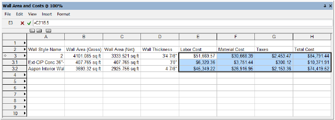
Add labels for columns E through H by typing names in the cells in row 2.
● In E2 enter Labor Cost
● In F2 enter Material Cost
● In G2 enter Taxes
● In H2 enter Total Cost
Click the following cells and enter the formula shown to determine the cost sums. Be sure to include the equal sign (=) before each item.
● In E3 enter =C3*15.5 (multiply the value in C3 by 15.5, the estimated rate of labor cost per area unit)
● In F3 enter =C3*9.2 (multiply the value in C3 by 9.2, the estimated material cost per area unit)
● In G3 enter =F3*.08 (multiply the value in F3 by 0.08, the estimated tax rate)
● In H3 enter =E3+F3+G3 (calculate the total cost of labor, material, and taxes)
Instead of entering the tax rate directly into the calculation, an alternative and more flexible approach is to set the tax rate in a separate spreadsheet cell and simply reference it in the calculation.
Format all of the cost data the same way. Select the four cost header cells (E3 through H3), and then right-click (Windows) or Ctrl-click (Mac) and select Format Cells from the context menu. The Format Cells dialog box opens. On the Number tab, select the options shown and click OK.
● Select Decimal
● In Dec. Places, enter 2
● Select Use Commas
● In Leader, enter $ (dollar sign)
Next, set up totals at the bottom of the columns as appropriate. The cells in the database header row (in this case, row 3) display sums for all of the database columns. Reference these database header row cells in spreadsheet cells to set up the totals.
To set up the totals:
Click the following cells and enter the formula shown to show sums from the database header row. Be sure to include the equal sign (=) before each item.
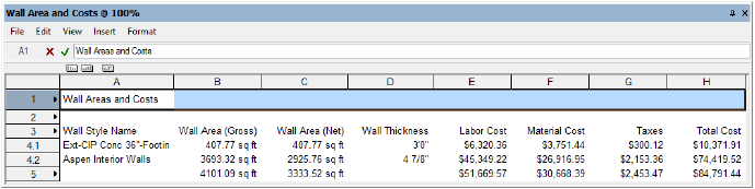
● In B4 enter =B3
● In C4 enter =C3
● In E4 enter =E3
● In F4 enter =F3
● In G4 enter =G3
● In H4 enter =H3
Select cells B4 and C4, right-click (Windows) or Ctrl-click (Mac), and select Format Cells from the context menu. On the Number tab, select Dimension Area and click OK.
Select cells E4 through H4, right-click (Windows) or Ctrl-click (Mac), and select Format Cells from the context menu. On the Number tab, select the options shown and click OK.
● Select Decimal
● In Dec. Places, enter 2
● Select Use Commas
● In Leader, enter $ (dollar sign)
Click cell A1 and enter Wall Areas and Costs as the schedule title.
Select row 2, right-click (Windows) or Ctrl-click (Mac), and select Insert Rows from the context menu to add an empty row between the schedule title and the column labels.
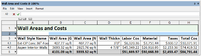
Select the empty rows at the bottom of the worksheet (6 through 11), right-click (Windows) or Ctrl-click (Mac), and select Delete Rows from the context menu.
Select View > Database Headers and then View > Grid Lines to hide the database header row and grid lines in the table.
Finally, select cells and use the Format Cells command to format the worksheet. You can change the font, font style, size, and color to format the text. Add cell borders, and change cell background color, as desired. Change the text alignment in cells, and resize rows and columns, if necessary.
See Formatting Worksheet Cells for details.
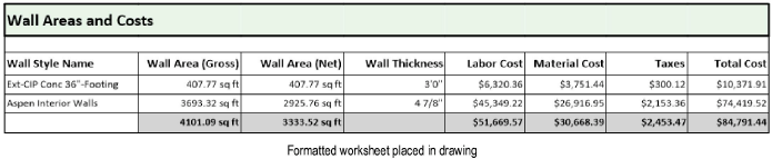
![]()