Worksheet window
The tool bar at the top of the worksheet window has several tools grouped into three tabs. Below the tool bar, the formula bar has controls that allow you to define the contents of the worksheet's rows and columns. The rows and columns display below the formula bar; right-click on a row number, column letter, or cell to open a context menu with additional commands.
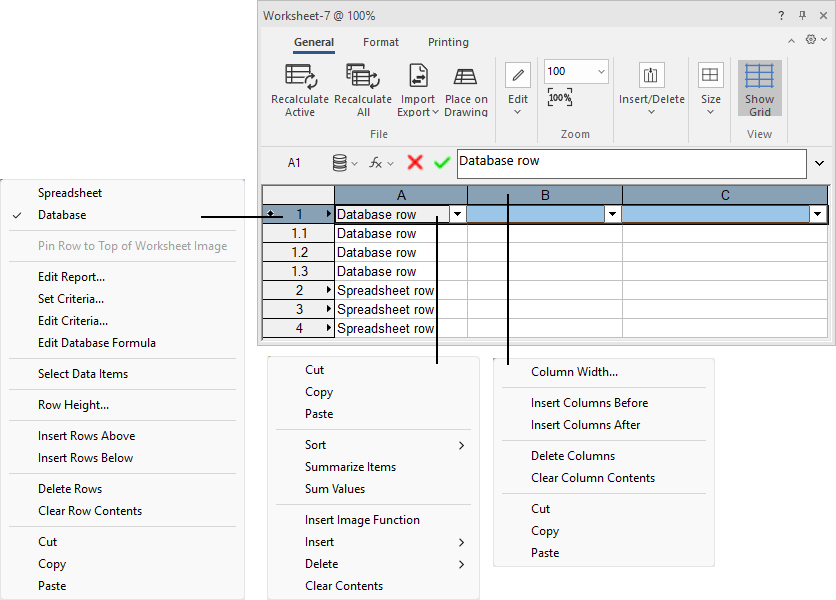
Left to right: row context menu, cell context menu, and column context menu
Worksheet: Overall controls
In the top right corner of the window, the following controls are always available.
Click to show/hide the controls.Click to show/hide the controls.
|
Control |
Description |
|
Minimize the Ribbon
|
On Windows, this button expands or collapses the tool bar. Alternatively, click (Mac) or double-click (Windows) a tab to expand or collapse the tool bar. |
|
|
Sets general worksheet options. Recalculate automatically: Recalculates all worksheet arithmetic functions when cells are edited. Set Default Font: Opens the Format Text dialog box to specify default formatting for the worksheet. Image Resolution: Set the resolution for worksheets with images (Vectorworks Design Suite product required). Resolutions higher than 150 DPI may increase file size significantly enough to affect performance. Show worksheet Tool bar group labels: Toggles the group labels on the tool bar on or off. |


Worksheet: General tab
Click to show/hide the tools.Click to show/hide the tools.
|
Tool |
Description |
|
Recalculate Active |
Recalculates the selected worksheet only, and updates it if it's referenced. Alternatively, right-click on the worksheet object in the drawing and select Recalculate Selected Worksheet, or click Recalculate from the Object Info palette of a selected worksheet. |
|
Recalculates all formulas in all worksheets, whether open or closed; also updates any referenced worksheets. Alternatively, right-click on the worksheet object in the drawing and select Recalculate All Worksheets. |
|
|
Import Export menu |
Import Worksheet: Opens a dialog box to import data; see Importing worksheets Export Worksheet: Opens a dialog box to export data; see Exporting worksheets Push Data to Excel File: For a worksheet referenced from an Excel file, updates the referenced file with changes you made in Vectorworks. See Microsoft Excel references. If the Excel file is open during this operation, you may need to close and re-open the file to see the changes. |
|
Place on Drawing |
Places an image of the worksheet on the drawing for display and printing. A preview of the worksheet image displays with the cursor; click to place the image where desired. See Placing a worksheet on the drawing. |
|
Cut |
Removes the contents of selected cells, temporarily storing the contents in the clipboard |
|
Copies the contents of selected cells to the clipboard, where they are temporarily stored; the original contents remain in the worksheet |
|
|
Places cell contents stored in the clipboard into the current cell or range of cells |
|
|
Clear Contents |
Deletes the contents of the selected cells |
|
Zoom level |
Displays the current zoom percentage; enter a percentage, or select one from the menu. Click the reset button Alternatively, roll the mouse wheel while holding Ctrl (Windows) or Option (Mac) to increase or decrease the zoom level by increments of 10%. This feature won't work properly if standard scrolling is disabled in the mouse setup. For example, if the mouse's scrolling size is set to "none," mouse zooming in the Vectorworks program is disabled. (The specific settings required for this feature depend on the type of mouse being used.) |
|
Rows menu |
Insert Rows Above and Insert Rows Below: Inserts rows in the worksheet, above or below the selected rows. The number inserted depends on how many rows in the worksheet are highlighted at the time the tool is selected. Delete Rows: Deletes the selected rows. To add rows to the bottom of the worksheet, click and drag the bottom right corner of the worksheet. Use caution when inserting or deleting rows. Depending on the type of cell references used in formulas, changes could affect the values returned by a formula. |
|
Columns menu |
Insert Columns Before and Insert Columns After: Inserts columns in the worksheet, to the left or right of the selected columns. The number inserted depends on how many columns in the worksheet are highlighted at the time the tool is selected. Delete Columns: Deletes the selected columns. To add columns to the right side of the worksheet, click and drag the bottom right corner of the worksheet. Use caution when inserting or deleting columns. Depending on the type of cell references used in formulas, changes could affect the values returned by a formula. |
|
|
Sets the height of selected cells in the specified units. Alternatively, drag the divider bar between the row numbers to adjust row height. |
|
|
Sets the width of selected cells in the specified units. Alternatively, drag the divider bar between the column letters to adjust column width. |
|
Auto Fit Height |
Sets the row height to automatically fit the contents of the selected cells |
|
Standard Width |
Applies the default width to the selected columns |
|
Show Grid |
Toggles the display of grid lines between the rows and columns in the worksheet window. If Pen attributes are applied to the worksheet object (from the Attributes palette), the grid in the worksheet image on the drawing is also affected. You can also apply Border formatting between rows and columns from the Format tab (see the section below). If you do so, turn off the Show Grid option. |
 to return to 100% zoom level.

Worksheet: Format tab
Set the appearance of worksheet cells with a variety of formatting options. Formatting applied to a database header row applies to all of the associated database sub-rows. The worksheet formatting also applies to worksheet images placed on a drawing.
You can apply Fill and Pen attributes to the worksheet image on the drawing (from the Attributes palette). However, it's not recommended to apply both cell formatting and attributes to the same object, because the results can be unpredictable.
Click to show/hide the tools.Click to show/hide the tools.
|
Tool |
Description |
|
Number Format |
Sets the number format for the selected cells. General: Specifies the default general format for any purpose Decimal: Uses decimal numbers; enter a value for the number of decimal places, and if desired, use commas as separators Scientific: Uses scientific numbers; enter a value for the number of decimal places Fractional: Uses fractional numbers; enter the rounding value for fractions Percentage: Uses percentages; enter a value for the number of decimal places Dimension: Uses dimension numbers Dimension Area: Uses the dimension area format (precision and units) as specified for this document; also displays the area units after the number Dimension Volume: Uses the dimension volume format (precision and units) as specified for this document; also displays the volume units after the number Angle: Determines the accuracy of angles and the measurement system used; the measurement system can be degrees/minutes/seconds, or decimal numbers up to eight decimal places Date: Uses date formats; select the desired format from the list Boolean: Evaluates the cell data to either True or False Text: Treats the cell contents as text, even if a number is in the character string Leader: Displays the specified leader text before the cell value (except for Boolean and Text formats) Trailer: Displays the specified trailer text after the cell value (except for Boolean and Text formats) |
|
Image Format (Design Suite product required) |
Sets the image format for the selected cells. See Inserting images in worksheet cells. Specify the type of image. 2D Attributes: Displays a rectangle with the same 2D attributes as the referenced object. For a styled wall, slab, or space, the rectangle fill is a top/plan cross-section view of the object. Thumbnail: Displays a thumbnail image of the referenced object in the cell; this is useful for 2D/3D symbols or plug-in objects. Use other settings to control the scale, view, rotation, and render mode shown in the thumbnail. Specify the size of the image. Auto size: Sizes the image automatically so that the entire image is always visible, even when the cell size changes. Fixed: Sizes the image according to the specified Height and Width; also specify the Units for the dimensions. Layer Scale: Sizes the image according to the scale of the layer on which the object appears (thumbnails only). Custom Scale: Select this option and then enter a scale for the image (thumbnails only). Specify the view details. Standard view: Select from any of the standard Vectorworks views for the image (thumbnails only). Render mode: For any view except Top/Plan, select the render mode for the image (Wireframe, Shaded, or Hidden Line); Top/Plan view is always rendered in Wireframe mode. Applies to thumbnails only. Component: Select which 2D/3D component view of symbols and plug-in objects to display in the worksheet cell; the options available depend on the Standard Views selection. Rotation: If Top/Plan view is selected, enter the number of degrees to rotate the image (thumbnails only). Margin: Enter the Size of the margin around the image, in the specified Units. |
|
Background fill style |
Sets the fill style for the background of the selected cells. No Fill: Removes all fill Solid Fill: Applies a fill of the selected color Pattern Fill: Applies a fill of the selected pattern, with the specified foreground and background colors |
|
Border |
Sets the borders for the selected cells. At the top of the popover, select the settings for line thickness, style, and color. Specify which parts of the selected cells to apply the settings to. No Border: Removes all borders Outline: Enables and disables borders on outside edges only Inside: Enables and disables borders on inside edges only The Custom Border is an interactive preview of the current settings. Click one of the displayed border lines to apply the current thickness, style, and color settings to that line only. |
|
Text options |
Sets the font, font size, color, and style of text in the selected cells. |
|
Alignment options |
Sets the horizontal and vertical alignment of text in relation to the cell border.
|
|
Merge cells
|
Merges a range of selected spreadsheet cells into one cell; cell and border formatting and text wrapping are applied to the cell group rather than to the individual cells. The cell contents and format of only the upper left cell in the group apply to the merged cells. Data and formatting in the other cells will be lost during the merge. To split merged cells, select the merged cell group and click the button again. |
|
Wrap text
|
Wraps text that exceeds the cell width (automatically adjusting row height); deselect to allow text that is longer than the cell width to "float" over empty adjacent cells. If adjacent cells contain content, unwrapped text may appear truncated. Numbers that exceed the cell width are displayed with # characters. |
|
Horizontal/vertical text
|
Orients text horizontally or vertically |
 : Text left and numbers right
 : Left
 : Right
 : Center horizontally
 : Text and numbers bottom
 : Bottom
 : Top
: Top : Center vertically


Worksheet: Printing tab
Click to show/hide the tools.Click to show/hide the tools.
|
Tool |
Description |
|
Print menu |
Print: Opens the Print dialog box, to print the current worksheet. This is the only way to print a worksheet unless the worksheet is placed on the drawing. Printer Setup: Opens the Printer Setup dialog box. This is almost identical to the standard Printer Setup dialog box, with the addition of Scaling options to help fit the worksheet on the printed page. Select how to fit the worksheet to the page; if Custom Scale is selected, specify the scale. All scaling is done symmetrically and maintains the aspect ratio. The setting is saved for each worksheet palette. Settings in this dialog box affect only the printer information for the worksheet. |
|
Page Margins |
Sets the units and margin sizes for printing |
|
Header/Footer |
Sets a header and footer for printing |
|
Print Tabs |
Includes the worksheet's column letters and row numbers in the printout |
|
Print Database Headers |
Includes the worksheet's database header rows in the printout |
Worksheet: Formula bar
Click to show/hide the controlsClick to show/hide the controls
|
Tool |
Description |
|
Active cell |
Displays the address of the active cell, such as A2 or F10 |
|
Database menu
|
The availability of these commands depends on how the worksheet is set up and which items are selected. Spreadsheet Row: Converts a database header row into a row of spreadsheet cells. This deletes all sub-rows and the information contained within them. Any formulas that were defined in the columns of the header row remain intact. This command has no effect on spreadsheet cells. Database Row: Converts a row of spreadsheet cells into a database header row and opens the Criteria dialog box (see The Criteria dialog box). This command has no effect on database rows. Show Database Headers: Toggles between displaying and hiding all worksheet database header rows in the worksheet window. Create Report/Edit Report: Opens the Create Report (spreadsheet row) or Edit Report (database header row) dialog box, to enter object selection criteria and data for a report; see Creating reports. Set Criteria: Opens the Criteria dialog box for setting new criteria that will be used to generate the database sub-rows (database header row only). Edit Criteria: Opens the Criteria dialog box for editing the criteria that were used to generate the database sub-rows (database header row only). Edit Database Formula: Displays the formula of the database row in the formula field, for editing. If the row is a spreadsheet row, it is converted into a database row. Select Data Items: Selects all objects on the drawing that meet the criteria for the database row (database header row) Select Item: When a sub-row is selected, selects an individual database object in the drawing |
|
Function menu
|
Insert Function: Opens the Select Function dialog box; select a function to be inserted in the formula (see Entering formulas in worksheet cells) Insert Criteria: Opens the Criteria dialog box to select search criteria to insert in a formula Insert Image Function: Inserts the image function in the formula for the current cell; see Inserting images in worksheet cells (Design Suite product required) |
|
Confirm/Cancel buttons |
|
|
Formula field |
Displays the constant value or formula for the active worksheet cell; see Entering constant values in worksheet cells and Entering formulas in worksheet cells. To expand or collapse the field, click the arrow to the right of the field, or drag the bottom border of the field up or down. |


 : Validates the entry in the Formula field; alternatively, press Enter.
 : Cancels the entry in the Formula field; alternatively, press Esc.
Worksheet: Row context menu
Most of the commands are also available on the worksheet tool bar or formula bar. The following commands are available only on the context menu.
Click to show/hide the commands.Click to show/hide the commands.
|
Command |
Description |
|
Pin Row to Top of Worksheet Image (Spreadsheet rows only) |
If the worksheet image in the drawing will be split horizontally, select this option for a spreadsheet row that you want to appear at the top of each image in a series of linked images. See Cropping or splitting worksheet images.
|
|
Select Item (Database sub-rows only) |
Selects an individual database object in the drawing |
Worksheet: Cell context menu
Most of the commands are also available on the worksheet tool bar or formula bar. The following commands are available only on the context menu.
Click to show/hide the commands.Click to show/hide the commands.
|
Command |
Description |
|
Sort |
Sorts the database sub-rows in ascending or descending order, according to the contents of the clicked column. The button on the database header cell displays an up or down arrow, along with a number that indicates the sort precedence for this column. The precedence is determined by the order in which you set the sorts. In each group of sub-rows, up to 20 columns can have a sort applied. This setting has no effect on image cells (Vectorworks Design Suite product required). |
|
Summarize Items |
Summarizes the database sub-rows according to the contents of the clicked column. Sub-rows that have identical items in this column are grouped together in a single row. The button on the database header cell displays a If all of the summarized sub-rows have the same value for one of the other columns, that value displays; otherwise "---" displays to indicate that the sub-rows have different values for that column. This setting has no effect on image cells (Vectorworks Design Suite product required). |
|
When rows are summarized, select this option for any columns whose values should be summed. The button on the database header cell displays a + symbol. For example, you might have a window schedule that sorts and summarizes the data by the Window ID column. Select Sum Values for the Price column to show the combined price of all windows with a particular ID. This setting has no effect on image cells (Vectorworks Design Suite product required). |
|
|
Pick Value from List (Design Suite product required) |
If the cell is in a database sub-row, and the column lists a field that only allows certain pre-defined values, use this option to edit the object's data. For example, you might want to change the sill style for several window objects from the window schedule. Select the sill cells for the objects to be changed, and right-click. Select a different sill type from the list of options to change both the worksheet and the objects' data records. |